Micro-Manager Imaging Software Guide
Dr. Matthew Köse-Dunn
TELEDYNE SCIENTIFIC CAMERAS
Introduction
Welcome to this guide on how to use Micro-Manager software with Teledyne Photometrics cameras! Micro-Manager is a free, open-source microscope control software plugin based inside ImageJ:
- Microscopes supported from every major brand
- Stages, piezos, filter wheels, shutters, and more specialist hardware also supported
- A vast library of ImageJ and Micro-Manager image analysis and acquisition plugins developed and maintained by a strong and diverse community of imaging users
- Built-in macro support and ability to write custom plugins
- Teledyne Photometrics Micro-Manager camera drivers are developed in-house so are always up to date with camera features, and well supported
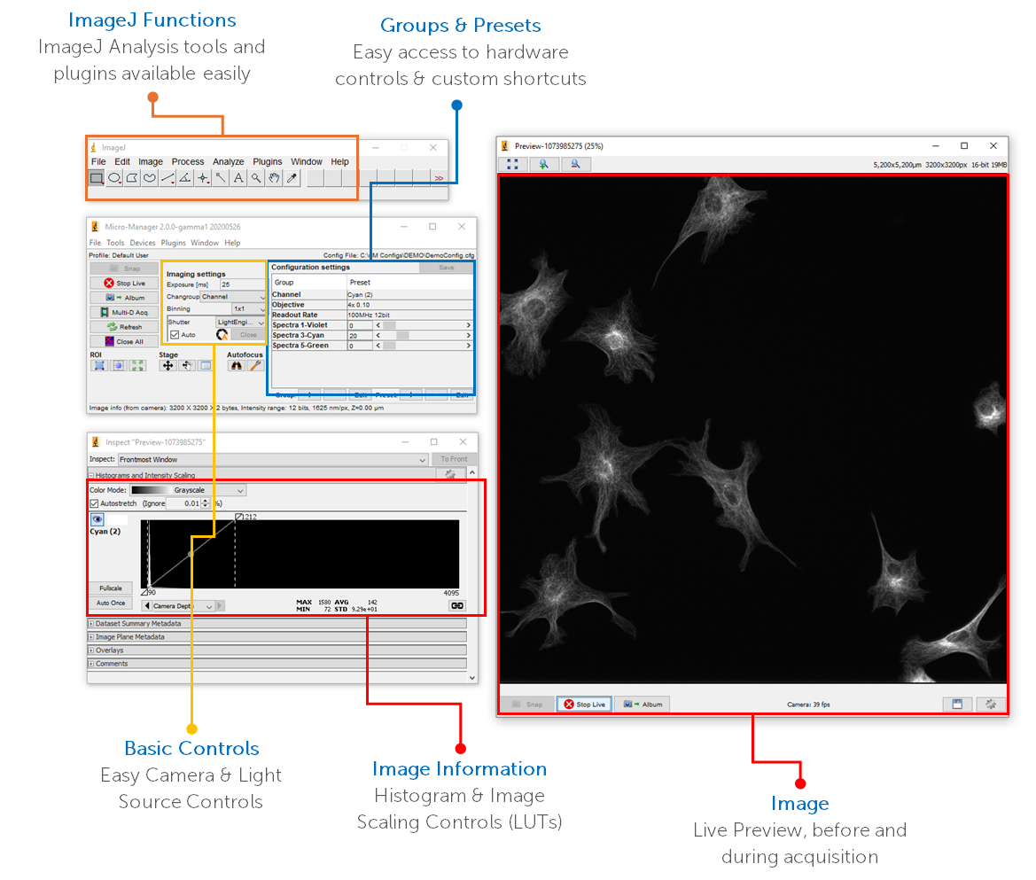
Figure 1: An overview of the Micro-Manager imaging software user interface, with different control areas highlighted.
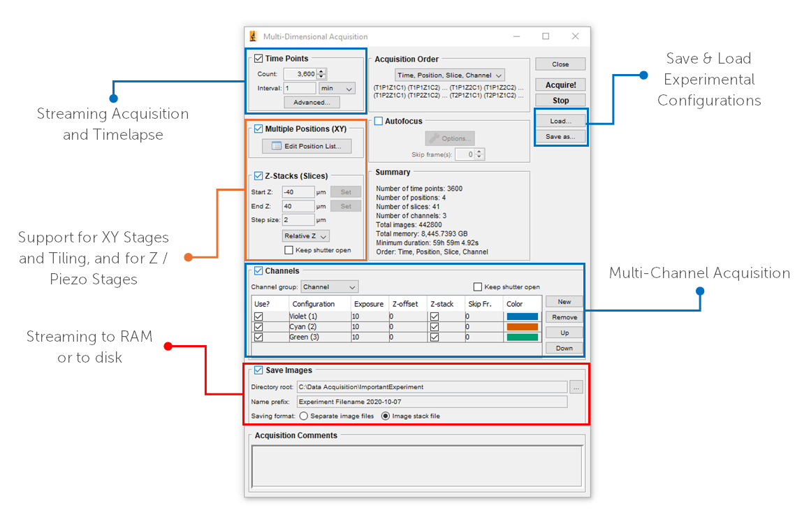
Figure 2: An overview of Micro-Manager multi-dimensional acquisition (Multi-D) which can control time points, multiple XY-Z positions, multiple wavelength channels, autofocus, acquisition order, and much more. Also controls saving to disk or streaming to RAM.
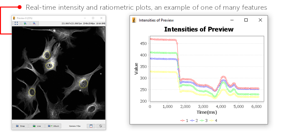
Figure 3: Another feature of Micro-Manager is real-time intensity and ratiometric intensity plots
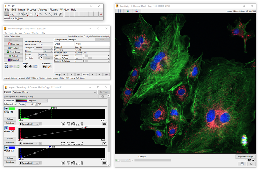
Figure 4: With Micro-Manager even the most complex imaging experiments are possible, automatable, and efficient.
Below are our suggested steps for how to begin using Micro-Manager and to make the most of your imaging system:
- Install your camera onto the microscope
- Connect the camera, and any other relevent imaging hardware, to the computer.
- Download and install PVCAM Drivers
- Download and install Micro-Manager
- Download or create a Hardware Configuration File to tell Micro Manager what hardware you’ll be using
- Create relevent 'Groups' and 'Presets' to control the necessary elements of your system
- Go ‘Live’ and start imaging!
This guide will take you through each of these steps in detail.
Installation
PVCAM
The first step to installing your Teledyne Photometrics camera and controlling it with Micro-Manager is to download the latest PVCAM drivers from our website. We have PVCAM versions for Windows or Linux systems, and frequently release new versions with updated features and support. There is also a SDK available for those who wish to customise their experience.
- Here is a link to download PVCAM: PVCAM DOWNLOAD
- Download and install PVCAM on your imaging PC
- Note: If your camera has a USB or PCIe interface and does not run on older Firewire interfaces, but you do have other firewire hardware such as older microscopes or devices, uncheck the two drivers containing ‘1394’, as these may conflict with other firewire devices. If you have no firewire devices, you do not need to change anything.
- Connect your camera power and data cables as directed in the camera manual
- Check your camera is recognised by the PC, either through 'Device Manager' on your start menu or by using the PVCAMTest utility that comes with PVCAM
- Once your PC recognises your camera, you're ready to go!
Micro-Manager
There are an enormous number of Micro-Manager versions available for download online. However, at any one time there is likely only one recommended version, that being the latest nightly build of Micro-Manager 2.0. Note: For some hardware and plugins other Micro-Manager versions may be required; please see the support pages for your hardware.
- Here is a link to download the latest nightly build of Micro-Manager for Windows or Mac: MICRO-MANAGER DOWNLOAD
- If using Windows, select the latest 64-bit version
- Download and install Micro-Manager on your imaging PC.
Hardware Configuration
With PVCAM your PC can talk to your Teledyne Photometrics camera, but you still need to tell Micro-Manager what imaging hardware you have available, especially if your microscope can be controlled by software. Compatible objectives, stages, light sources and more can all be controlled via Micro-Manager, once added to a Hardware Configuration File along with your camera.
Hardware Configuration Files are created and edited via the Hardware Configuration Wizard. On your first time opening Micro-Manager you’ll need to create this config file, but every subsequent time you open Micro-Manager this file will be pre-loaded and ready to go. You can also modify existing files, such as adding a new piece of hardware, or download pre-made config files.
Creating a new Hardware Configuration File
1. Make sure your camera and any additional imaging hardware is powered on and successfully connected to the computer.
2. Open Micro-Manager, you will be presented with the startup screen (Fig.5). Change the 'Hardware Configuration File' dropdown to (none). This will let you set up your own config file, the other option is a software demo.
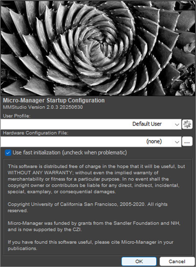
Figure 5: The initial Micro-Manager startup screen.
3. This is Micro-Manager (Fig.6). At first there will be two windows, one for ImageJ, and another for your version of Micro-Manager. All functions of typical ImageJ can be used during Micro-Manager use, such as image analysis, processing, measurements, custom plugins, etc. At the moment the Micro-Manager window is mostly blank, the first thing to do is tell it what image software you have by creating a new Hardware Configuration File.
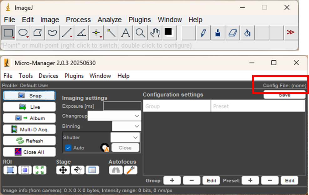
Figure 6: The initial Micro-Manager user interface. No groups/presets have been installed, and there is no Hardware Configuration File (as highlighted by the red box).
4. Go to 'Devices' and choose 'Hardware Configuration Wizard'
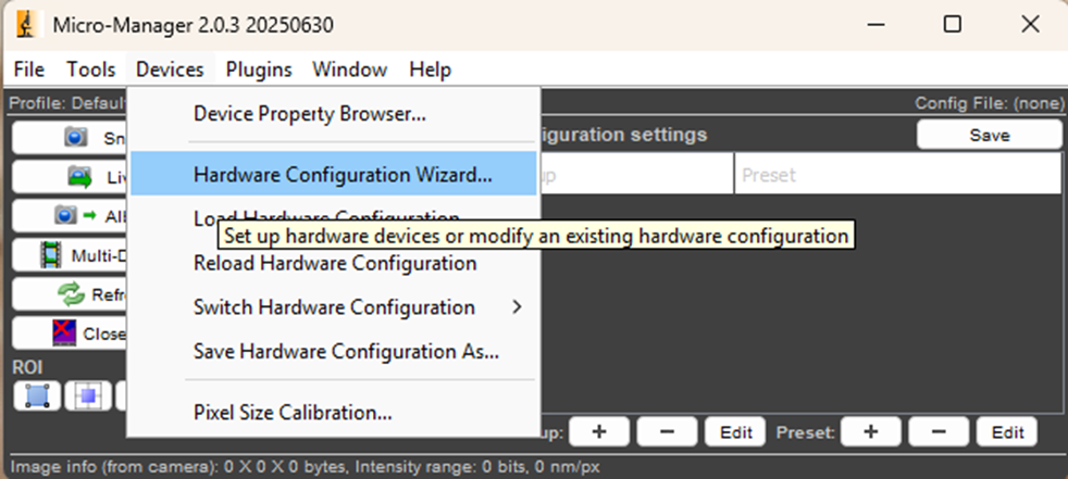
Figure 7: Select 'Devices' and 'Hardware Configuration Wizard' to make your Hardware Configuration File.
5. Select 'Create new configuration' and 'Next'
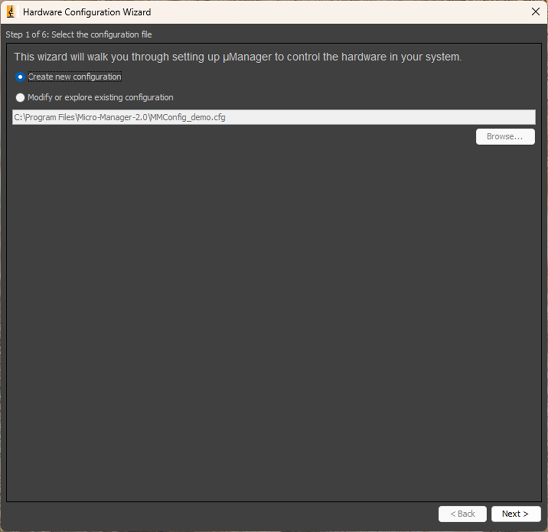
Figure 8: Select 'Create new configuration' and 'Next'
6. On this page (Fig.9) you can add or remove your imaging hardware. If your camera, light source, etc. isn't added to the list on this page, Micro-Manager won't recognise or be able to control them. Under 'Available Devices' is an alphabetical list of imaging hardware vendors. Find your device folder, select the relevent device, and select 'Add'. You'll be prompted to name the device, and after a delay it will be added to the list above.
Note: Most devices have an online help and installation guide, which can be found through selecting the device and clicking ‘Help’.
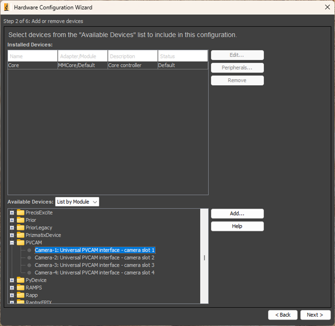
Figure 9: Select the relevent Available Devices for Micro-Manager to recognise and control.
7. Teledyne Photometrics cameras are listed under ‘PVCAM’. There are up to four camera slots that you can use. If you have only one camera connected, this will always be ‘Camera-1’. If your Micro-Manager says 'PVCAM (unavailable)' you still need to install PVCAM and restart Micro-Manager
8. Once you have added all your necessary imaging hardware, advance the Hardware Configuration Wizard to the end and click 'Finish'. Some hardware may have further configuration steps, but for PVCAM Cameras, no further steps are necessary!
9. The final step will invite you to name and save your Hardware Configuration File. This will be saved by default to the Micro-Manager installation folder within C:\Program Files, and will be pre-selected every time you use Micro-Manager. You can make a number of different config files for different imaging setups or camera combinations, just make sure you know where they are saved.
Adding a Manual Objective Turret
Micro-Manager supports automated objective turrets for many microscopes. However, for manual microscopes, a manually changed objective or magnification indicator can be added in, which can be used to record which objective was used, and provide automatically updating pixel scaling information.
1. In the Available Devices list on the Hardware Configuration Wizard, locate the ‘DemoCamera’ folder and add ‘DHub’.
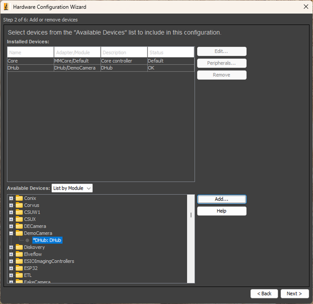
Figure 10: Select 'DemoCamera' and 'DHub'.
2. A Peripheral Devices Setup window will then appear – within this, select ‘DObjective’. This will add a dummy/demo objective to the device configuration. The same can be done for the other components in the peripheral list.
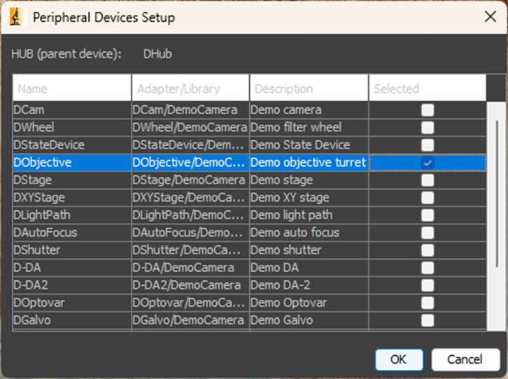
Figure 11: This is a list of all Demo/Dummy (D) devices available. Select 'DObjective'.
3. Advance the wizard to Step 3 of 6 and untick 'Use autoshutter by default'
4. Advance the wizard to Step 5 of 6, where you can set the label for each of your objectives according to their magnification, NA etc.
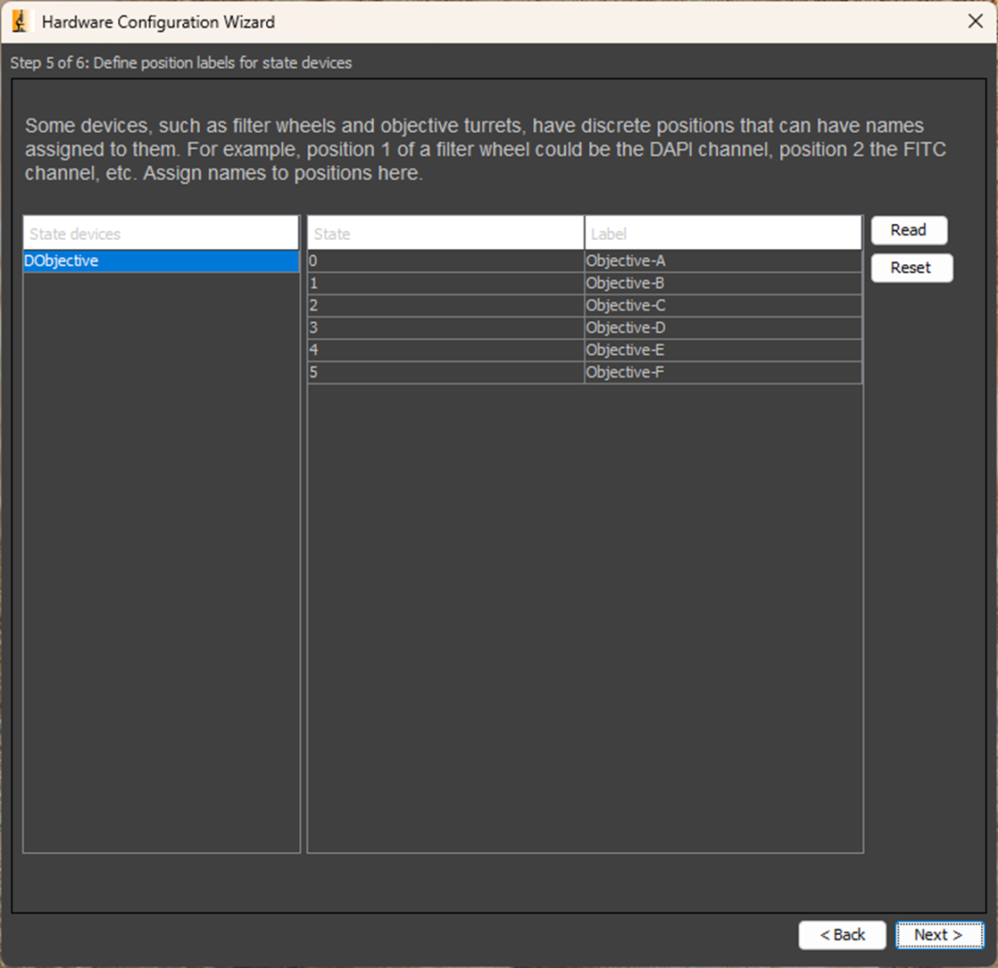
Figure 12: Enter the details of each of your manual microscope objectives in order to apply pixel scaling information.
5. Finish the wizard and add a group for ‘Objective’ as described in the Groups and Presets section below.
6. You can now set up Pixel Scaling Information following the instructions on that section below.
Installing other microscope hardware
Light Sources: Micro-Manager can control light sources from many manufacturers. Some example installation guides are linked below:
CoolLED pE300, pE340 and pE4000 Light Sources
Lumencor SPECTRA, SPECTRA X, AURA and CELESTA Light Engines
Full Support List: For a list of supported hardware in Micro-Manager, complete with installation guides for devices, please see the following web page:
Micro-Manager Device Support List
Note:For some hardware, additional files and drivers may be needed from the device manufacturer. Please see the website for your device manufacturer or contact their support teams.
Which hardware is on which port?
Please note, whenever adding any hardware to Micro-Manager using USB interfaces, you will need to check which COM port each device is assigned to in order for them to function as intended. To find out which device is connected to which COM port please refer to the ‘Device Manager’ in Windows:
- In Windows 10/11 right click the start button and select ‘Device Manager’
- Look at ‘Ports (COM & LPT)’ in the Device Manager to see your connected hardware (if connecting them via USB)
- In order to determine which device is on which port you may need to unplug the device and then go to ‘Action’ and ‘Scan for hardware changes’ to see which device is no longer present.
- Once you know which device is on which COM port, select this port when adding the device to Micro-Manager
Hardware Setup
Now that you've created a Hardware Configuration File you can start to add groups and presets in order to control your recognised imaging hardware and make your imaging more powerful and efficient.
Groups and Presets
In Micro-Manager, we can make shortcuts to any hardware controls that will be frequently used. These are called ‘Groups’ and drastically increase your imaging efficiency, as everything you need to control about your imaging setup can be accessed all in one place. Each Group can control a single setting (e.g. camera imaging mode) or multiple (e.g. which filter wheel is in the light path).
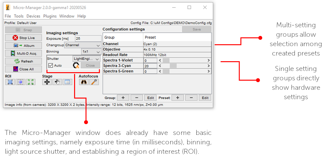
Figure 13: Details on using Groups and Presets.
Single Setting Groups
Single setting groups will provide direct access to a hardware control, such as a camera readout mode, light source intensity, or microscope objective turret position. Most groups you make will likely be single setting groups. These come in the form of dropdown menus, some are simply ON/OFF toggles. Here's how to create a single setting group:
1. Click the plus (+) button next to ‘Group’ in order to add a new group. If you want to remove or edit a group, use the minus (-) or 'Edit' buttons respectively (but not the buttons to the right in the Preset section)
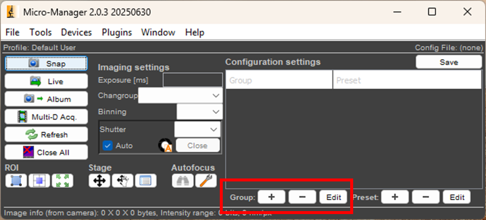
Figure 13: Group Controls. To add a new group, use the plus button.
2. The Group Editor menu will appear, showing a list of every setting for all available hardware, listing each piece of hardware in alphabetical order (depending on how you named the hardware when using the Hardware Configuration Wizard). Note: Fig.14 below is from a demo version and shows no hardware, if you see a screen similar to this please repeat the Hardware Configuration File setup steps or check your Device Manager.
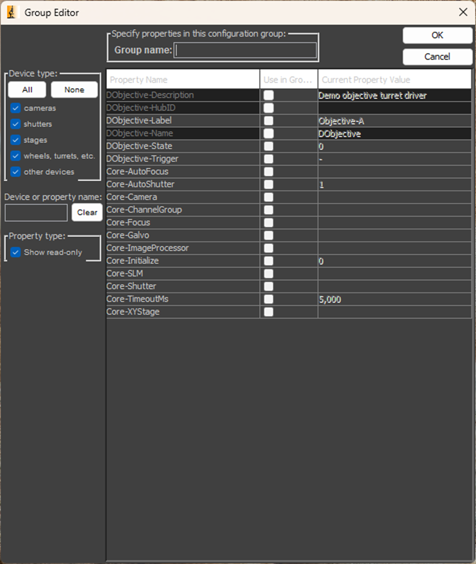
Figure 14: Group Editor. If yours looks like this, no imaging hardware has been properly recognised.
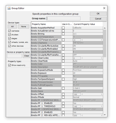
Figure 15: Group Editor. This is from an instance of Micro-Manager with a Kinetix sCMOS camera added to the config file, so all of the available Kinetix settings are in this list to add to a group for modification and control.
3. Find the setting that you want and check the box next to it. Be sure to only select one setting at a time.
4. Name the group with a name that makes sense to you (‘Fan speed’ for a group that controls camera fan speed, for example), and click OK.
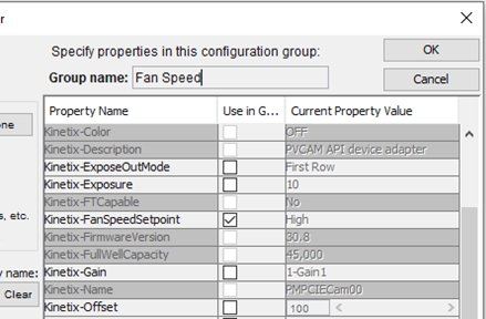
Figure 16: Check one setting at a time, then give it a relevant name.
5. You will now have a group that allows you to directly change that hardware setting, in this case, Fan Speed. Click the dropdown to control the setting.
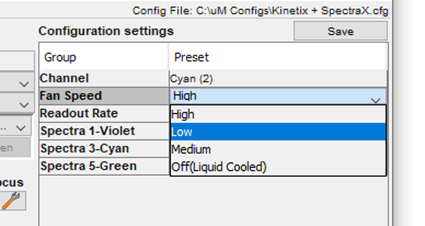
Figure 17: The Fan Speed group has been added to the Micro-Manager window.
6. Repeat these steps to add a Group fo revery setting you want to modify when imaging.
Multiple Setting Groups
Sometimes changing a hardware state in the system requires multiple individual components to be changed. For example, to change the illumination channels on your light source, you’ll need to select multiple settings such as the ‘Violet’ and ‘Cyan’ channels in order to switch between them, and not have both active at the same time. You'll also want to control the intensity of these channels. This is where multiple-setting groups come in.
In Micro-Manager, we can create groups that control multiple settings, and then create presets that specify the value of each setting. In the case of the Channel group, we would create one preset per wavelength channel – Brightfield can also be included if your microscope has computer-controllable brightfield lamp and shutters. Here's how to create a multi-setting group:
1. Click the plus (+) button next to ‘Group’ in order to add a new group. If you want to remove or edit a group, use the minus (-) or 'Edit' buttons respectively (but not the buttons to the right in the Preset section)
Figure 18: Group Controls. To add a new group, use the plus button.
2. Identify the settings you want to change in the Group Editor menu, and then select every box next to all the hardware settings that need to change. In this case, each different wavelength channel you want to use from your light source.
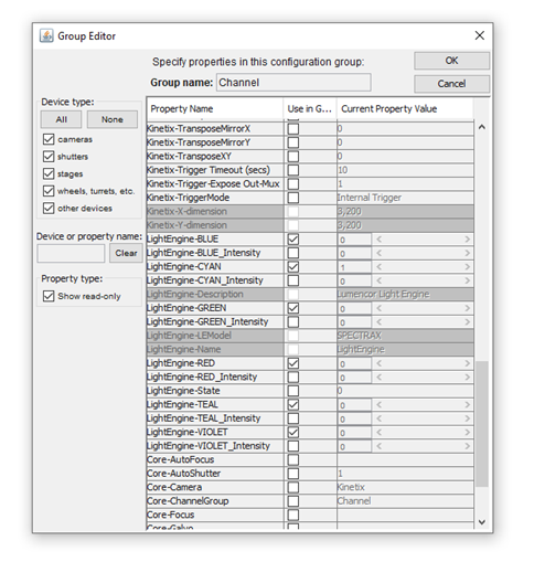
Figure 19: The Group Editor. For a multi-setting group, select every relevent box. In this example, we selected all the wavelength channels of our light source.
3. Give this group a name that makes sense and click OK. This multi-setting group will require several presets in order for you to control each setting within the group. When you click OK, the ‘Preset Editor’ window will appear. Each preset is a setting within the group, for example if your group contains multiple illumination channels, each preset would have one channel on and all the other channels off. Switching between these presets would then cycle between the illumination channels.
4. Make the first preset for this group in the preset editor window. Note: changing settings here will change the physical hardware state, so be aware parts may move or activate.
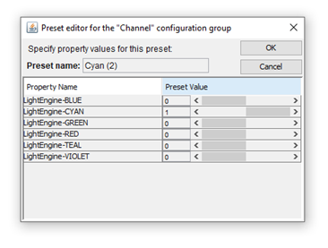
Figure 20: The Preset Editor. This will appear when first adding a multi-setting group. Select a single setting, you'll add the others later using Preset controls.
5. Once your first preset is created, you’ll be back at the Micro-Manager window. Select the multi-setting group you created, and then click the plus button in the Preset controls (next to the group controls) to add a new Preset for all remaining options required.
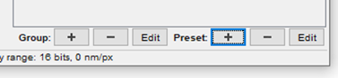
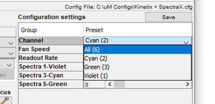
Figure 21: In order to control each setting of your new multi-setting group, select the plus (+) button on the preset menu and select one setting. Repeat this for every permutation desired.
Startup Configuration Settings
When Micro-Manager is closed, the values in the Groups list and in the Device Property Browser are not stored, they will go to their default values the next time Micro-Manager is loaded. To avoid this and specify which values your settings should be on startup, or even on shutdown, Micro‑Manager has a special Group called ‘System’. Here's to set default startup parameters for your hardware:
- Create a new Group as described above, called ‘System’. Select every hardware option that you would like to set a Startup or Shutdown value for.
- In the preset editor, for Startup values name the preset ‘Startup’, and set the values.
- To add a Shutdown preset, create a new preset as described above, naming it ‘Shutdown’, and set the values appropriately.
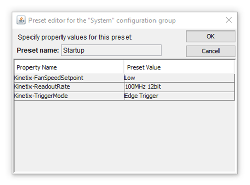
Figure 22: Use Groups and Presets to ensure your Micro-Manager config doesn't change when you shutdown your PC
Pixel Scaling Calibration
To allow XY scaling information in images and the inclusion of scale bars, you must set up your Pixel Size Calibration. This requires either a manual objective turret to be included in your Hardware Configuration File (as described earlier), or an automated objective turret controlled in Micro-Manager. Here's how to set up Pixel Scaling Calibration:
1. Under ‘Devices’, select ‘Pixel Size Calibration’.
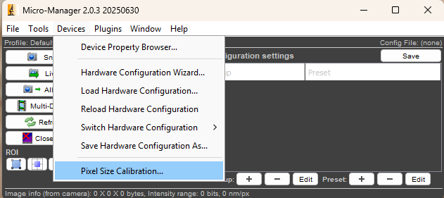
Figure 23: Pixel Size Calibration can be found in the Devices menu.
2. The Pixel Size Calibration Window will appear, select ‘New’. To open the Pixel Config Editor. This is where all hardware that affects magnification (objectives, optivars, multiple cameras) can be selected though ticking the ‘Use in Group’ checkbox.
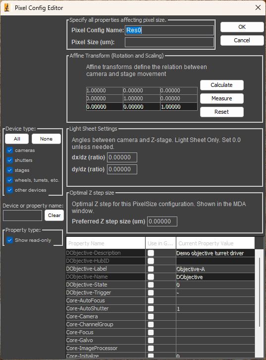
Figure 24: The Pixel Config Editor allows users to select any hardware that may affect the magnification.
3. Set an initial value for a pixel configuration (for example, setting your Objective turret to ‘10x’), and give this pixel configuration a corresponding name “10x”.
4. Calculate and enter the resulting image pixel size in micrometers based on the following formula, including any C-mount / optical tube magnification in the system:
Image Pixel Size = (Camera Pixel Size) / (Objective Magnification × Additional Magnification)
You can find your camera pixel size on your Camera Specification Sheet, or in the following table:
| Teledyne Photometrics Camera | Pixel Size |
| Kinetix/Kinetix22 | 6.5 μm |
| Prime BSI/BSI Express | 6.5 μm |
| Prime 95B | 11 μm |
| Moment/Retiga E7 | 4.5 μm |
| Retiga E9 | 3.67 μm |
| Retiga E20 | 2.4 μm |
| Iris 9/15 | 4.25 μm |
5. Once you have inserted your pixel size, click ‘Calculate’. Alternatively, if you have a correctly calibrated, motorized XY stage installed into Micro-Manager you can click ‘Measure’ for an automated measurement of pixel size.
6.Click ‘OK’, and then repeat the process for all remaining objectives, or permutations of different magnification-adjusting hardware.
7. Once you have finished adding these, click ‘Close’ and you will be prompted to save the changes you have made into the Hardware Configuration File.
Hardware Timestamps
Many cameras from Teledyne Photometrics are able to provide highly accurate and precise hardware timestamps, generated by the camera’s onboard processor. This will be the most precise timestamp available for when an image was taken. These can be enabled within Micro-Manager, and will then be included in all streaming acquisitions (i.e., anything but pressing ‘Snap’). Here's how to enable and view Hardware Timestamps:
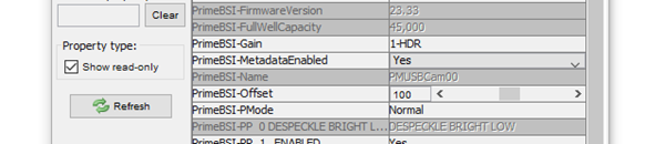
1. In the Device Property Browser or by creating a group, find the property ‘[Camera Name]‑MetadataEnabled’, and select ‘Yes’.
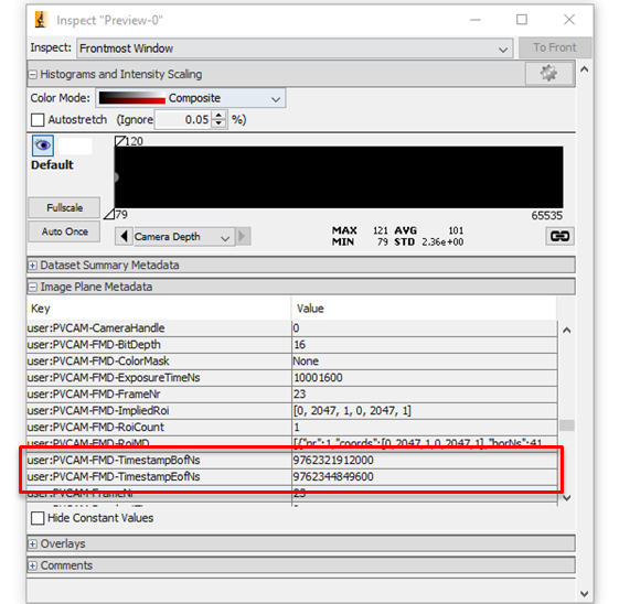
2. Now each acquired image will show additional metadata under the ‘Image Plane Metadata’ tab of the Inspect window, starting with “PVCAM-FMD” (“Frame Meta Data”).
3. This metadata includes many additional items, the hardware timestamps are under the name “PVCAM-FMD-TimestampBofNs” and “…EofNs”, meaning “Beginning of frame, Nanoseconds” and “End of frame” respectively. These two times will differ by the frame roll time for rolling shutter cameras, and are in units of 1 ns, with 100 ns precision and 1 line time accuracy (10-20 μs, depending on camera speed).
Simultaneous Multichannel Imaging Setup
Running two or more PVCM Cameras simultaneously
Micro-Manager is capable of running up to 4 PVCAM cameras simultaneously. The only requirement is that the cameras have the same sensor size or region of interest applied, and the same bit depth of resulting images. The below guide is for the specific case where the cameras will be run simultaneously; if you want to install and access multiple cameras without simultaneous use, follow only steps 1, 2 and 6.
Here's how to set up multiple PVCAM cameras in Micro-Manager:
1. Create a new configuration file or edit an existing one. When adding available camera hardware,add in each of the Camera-1, Camera-2 etc. (up to 4) PVCAM camera slots that you are using and name them appropriately (especially if using multiples of the same camera model). These should all appear in the Installed Devices list with a status of ‘OK’.
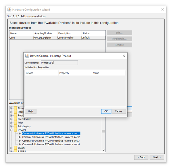
Figure 25: Adding multiple PVCAM cameras to the Hardware Configuration Wizard.
2. Now we add in a special ‘Multi Camera’ Utility to treat multiple cameras as one multichannel camera device for simultaneous acquisition. Go to the ‘Utilities’ folder and add ‘Multi Camera’.
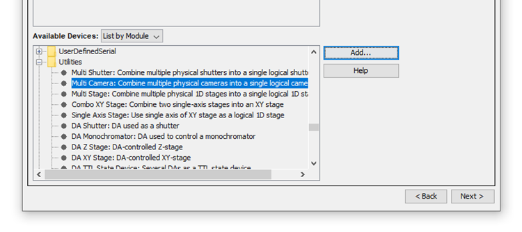
Figure 26: Go to the Utilities folder in the Available Devices list and select 'Multi Camera'.
3. Now finish off your Hardware Configuration File. Once your file is completed and loaded, you may see a ’Circular buffer can’t be started’ error, ignore this, as we need to inform the Multi Camera utility which devices to use. Go to ‘Devices’, open ‘Device Property Browser’ and find ‘Multi Camera-Physical Camera 1’. Choose the appropriate camera for each of these labelled 1 through 4.
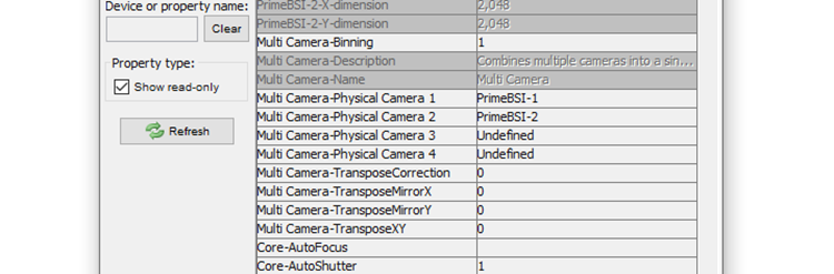
Figure 27: Go to 'Devices' menu, select 'Device Property Browser' and change 'Multi Camera-Physical Camera X' to the relevent camera models.
4. Now create a Group for Core-Camera as described in ‘Groups and Presets’.
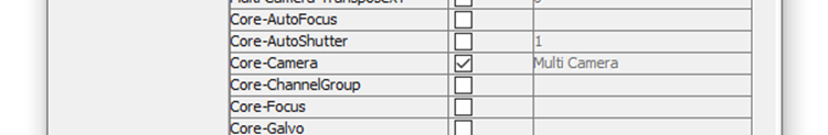
Figure 28: Select the plus (+) group button and add 'Core-Camera' as a group.
5. In the Core Camera group in the Micro-Manager window, select ‘Multi Camera’ from the dropdown to view simultaneous output.
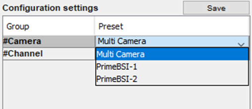
Figure 29: Select 'Multi Camera' from your new Core-Camera group
6. Hit ‘Live’ to image in multiple colors simultaneously. You may need to set up your image display settings to view a composite image. In the Inspect window under ‘Histograms and Intensity Scaling’, choose ‘Color Mode: Composite’. Choose the appropriate color for each channel by clicking the rectangle next to the eye symbol for each histogram, shown below in green and red. The eye symbol will toggle that channel’s visibility.
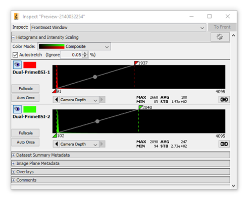
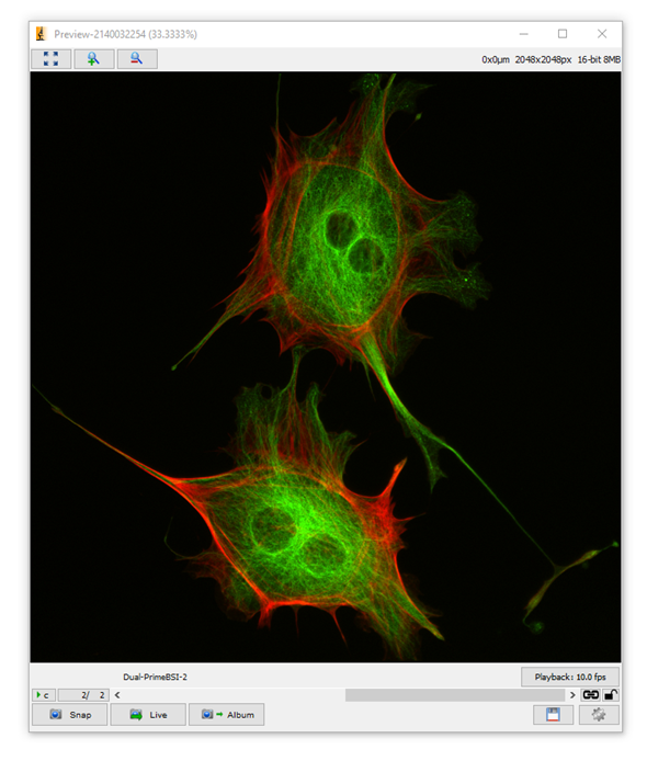
Figure 30: Simultaneous multi-camera imaging in the Preview window. To select the correct false colours for your channel wavelengths, use the histogram settings.
Using a single PVCAM camera with an image splitter for simultaneous imaging
Micro-Manager also supports using single camera image splitters, where separate wavelengths are directed onto separate portions of a single camera sensor. This requires a separate piece of imaging hardware known as an image splitter. Any combination of horizontal and vertical splits is possible, splitting each dimension 2, 3 or 4 ways. Commonly a 2-way or 3-way vertical split, or a combined 2-way vertical and 2-way horizontal split is used. For advice on how to align splitting devices, please see manufacturers’ instructions.
Here's how to setup an image splitter in Micro-Manager:
- Align your splitter according to manufacturer’s instructions. In the case of a 2-way or 3-way single direction split, for rolling shutter cameras it is most advantageous to align the channels vertically (Fig.31, left)
- In Micro-Manager, open ‘Plugins / On-The-Fly Image Processing / Split View’ to add one direction of split, specifying how many times the view is split in this dimension (Fig.31, center top)
- To add further splits in the opposing direction, in the ‘On-The-Fly Processor Pipeline’ Window, click ‘Add’ and select ‘Split View’.
- Hit ‘Live’ to image in multiple colors simultaneously (Fig.31, right).
- You may need to set up your image display settings to view a composite image. In the Inspect window under ‘Histograms and Intensity Scaling’, choose ‘Color Mode: Composite’. Choose the appropriate color for each channel by clicking the rectangle next to the eye symbol for each histogram, shown below in green and red. The eye symbol will toggle that channel’s visibility.
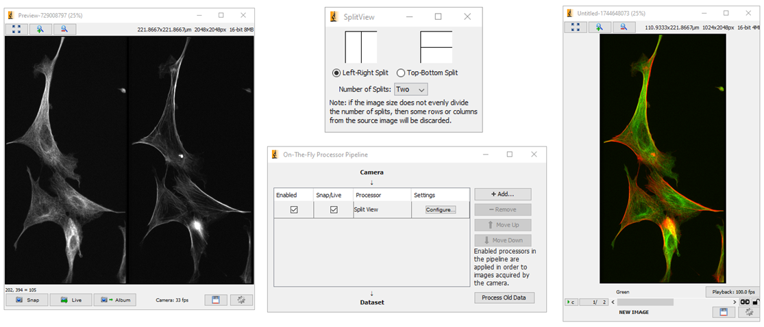
Figure 31: Setting up an image splitter with Micro-Manager. Left and right windows show the split and combined image previews (each half of the camera sensor detecting a different wavelength).
Important Settings for PVCAM Cameras
In order to get the most out of your Teledyne Photometrics PVCAM camera, each camera model has specific settings to optimise your imaging experience. Here are lists for each of the major product families, namely the Kinetix Family, the Prime BSI Family and the Prime 95B.
Kinetix Family (Kinetix and Kinetix22)
|
|
Camera Setting |
Setting Name in list |
Values |
|
Essential |
Mode – Change between the four imaging modes of the Kinetix. This changes both the readout and gain, which are optimized for each mode. |
Port |
‘Speed’ – 8-bit, 498 fps across full sensor ‘Sensitivity’– 12-bit, 88 fps across full sensor, low read noise mode at speed ‘Dynamic Range’ – 16-bit, 83 fps across full sensor, large full well capacity for imaging intense signals ‘Sub-Electron’ – 16-bit, 5 fps across full sensor, ultra-low read noise of 0.7 e- |
|
Recommended |
Metadata – Additional hardware metadata including Timestamps |
MetadataEnabled |
‘Yes’ – Add additional hardware metadata including a 10ns precision timestamp for the beginning and end of each frame |
|
Fan Speed – Control over air cooling fan speed |
FanSpeedSetpoint |
‘Low’ – For air cooling for typical (< 2 seconds) exposure times and room temperatures, camera airflow unobstructed. ‘High’ – Air cooling with long exposures or in confined or warm environments ‘Off’ – Use only when water cooling is in use |
|
|
Triggering |
Trigger In – Hardware trigger to control camera acquisition |
TriggerMode |
‘Internal’ – Camera runs on own internal timing as defined by software. Other modes allow external control of camera. Please see camera manual for explanation of other trigger modes. |
|
Expose Out Trigger Behavior |
ExposeOutMode |
Used when synchronizing external hardware through hardware triggering. Please see camera manual for explanation of the options. |
|
|
Number of Expose Out Cables Used |
Trigger - ExposeOutMux |
If using Multi Expose Outs to trigger multiple light sources etc., how many cables to use |
|
|
Advanced |
SMART Streaming Enable – Use for faster sequential multi-channel acquisitions with channel-dependent exposure times |
SMARTStreamingEnabled |
‘No’ – Don’t use SMART Streaming ‘Yes’ – Use SMART Streaming. Please see camera manual for instructions on SMART Streaming and when to use it. |
|
SMART Streaming Exposure Times – list of exposure times to use for above feature |
SMARTStreamingValues |
List of exposure times to use, separated by semicolons ; |
Prime BSI Family (Prime BSI and Prime BSI Express)
|
|
Camera Setting |
Setting Name in list |
Values |
|
Essential |
Readout Mode – Main camera mode setting |
ReadoutRate |
‘200MHz 12 Bit’ - Low light / high speed imaging ‘100MHz 16 Bit’ - High dynamic range imaging |
|
Gain 100MHz – Conversion factor between photoelectrons signal and grey levels displayed |
Gain – Create this group after setting ‘Readout Rate’ to ‘100MHz 16 Bit’ (both modes required) |
‘CMS’ – Recommended for all low light imaging. Low read noise mode. ‘HDR’ – For imaging bright and dark things simultaneously. Maximum dynamic range. |
|
|
Gain 200MHz – Conversion factor between photoelectrons signal and grey levels displayed |
Gain – Create this group after setting ‘Readout Rate’ to ‘200MHz 11 Bit’ (both modes required) |
For practically all low-light or fluorescence imaging: ‘3-Sensitivity’ For brightfield imaging: ‘1-Full Well’ or ‘2-Balanced’ |
|
|
Recommended |
Metadata – Additional hardware metadata including Timestamps |
MetadataEnabled |
‘Yes’ – Add additional hardware metadata including a 10ns precision timestamp for the beginning and end of each frame |
|
Fan Speed – Control over air cooling fan speed |
FanSpeedSetpoint |
‘Low’ – For air cooling for typical (< 2 seconds) exposure times and room temperatures, camera airflow unobstructed. ‘High’ – Air cooling with long exposures or in confined or warm environments ‘Off’ – Use only when water cooling is in use |
|
|
Triggering |
Trigger In – Hardware trigger to control camera acquisition |
TriggerMode |
‘Internal’ – Camera runs on own internal timing as defined by software. Other modes allow external control of camera. Please see camera manual for explanation of other trigger modes. |
|
Expose Out Trigger Behavior |
ExposeOutMode |
Used when synchronizing external hardware through hardware triggering. Please see camera manual for explanation of the options. |
|
|
Prime BSI Only Number of Expose Out Cables Used |
Trigger - ExposeOutMux |
If using Multi Expose Outs to trigger multiple light sources etc., how many cables to use |
|
|
Advanced |
Prime BSI Only SMART Streaming Enable – Use for faster sequential multi-channel acquisitions with channel-dependent exposure times |
SMARTStreamingEnabled |
‘No’ – Don’t use SMART Streaming ‘Yes’ – Use SMART Streaming. Please see camera manual for instructions on SMART Streaming and when to use it. |
|
Prime BSI Only SMART Streaming Exposure Times – list of exposure times to use for above feature |
SMARTStreamingValues |
List of exposure times to use, separated by semicolons ; |
Retiga E Family (Retiga E7, Retiga E9, Retiga E20)
|
|
Camera Setting |
Setting Name in list |
Values |
|
Essential |
Readout Mode – Main camera mode setting |
ReadoutRate |
Differs between models, for the Retiga E7: ‘Speed’ – High-speed imaging |
|
Recommended |
Metadata – Additional hardware metadata including Timestamps |
MetadataEnabled |
‘Yes’ – Add additional hardware metadata including a 10ns precision timestamp for the beginning and end of each frame |
|
Triggering |
Trigger In – Hardware trigger to control camera acquisition |
TriggerMode |
‘Internal’ – Camera runs on own internal timing as defined by software. Other modes allow external control of camera. Please see camera manual for explanation of other trigger modes. |
|
Expose Out Trigger Behavior |
ExposeOutMode |
Used when synchronizing external hardware through hardware triggering. Please see camera manual for explanation of the options. |
Prime 95B
|
|
Camera Setting |
Setting Name in list |
Values |
|
Essential |
Readout Mode – Main camera mode setting |
ReadoutRate |
‘200MHz 12 Bit’ - Low light / high speed imaging ‘100MHz 16 Bit’ - High dynamic range imaging |
|
Gain – Conversion factor between photoelectrons signal and grey levels displayed |
Gain – Create this group after setting ‘Readout Rate’ to ‘200MHz 12 Bit’ |
For practically all low-light or fluorescence imaging: ‘3-Sensitivity’ For brightfield imaging: ‘1-Full Well’ or ‘2-Balanced’ |
|
|
Clearing – Antiquated setting regarding charge clearance |
ClearMode |
‘Never’ – For all imaging. Other settings may introduce framerate and timing delays. This may require setting on startup. |
|
|
Recommended |
Metadata – Additional hardware metadata including Timestamps |
MetadataEnabled |
‘Yes’ – Add additional hardware metadata including a 10ns precision timestamp for the beginning and end of each frame – see Page 26. |
|
Fan Speed – Control over air cooling fan speed |
FanSpeedSetpoint |
‘Low’ – For air cooling for typical (< 2 seconds) exposure times and room temperatures, camera airflow unobstructed. ‘High’ – Air cooling with long exposures or in confined or warm environments ‘Off’ – Use only when water cooling is in use |
|
|
Triggering |
Trigger In – Hardware trigger to control camera acquisition |
TriggerMode |
‘Internal’ – Camera runs on own internal timing as defined by software. Other modes allow external control of camera. Please see camera manual for explanation of other trigger modes. |
|
Expose Out Trigger Behavior |
ExposeOutMode |
Used when synchronizing external hardware through hardware triggering. Please see camera manual for explanation of the options. |
|
|
Number of Expose Out Cables Used |
Trigger - ExposeOutMux |
If using Multi Expose Outs to trigger multiple light sources etc., how many cables to use |
|
|
Advanced |
SMART Streaming Enable – Use for faster sequential multi-channel acquisitions with channel-dependent exposure times |
SMARTStreamingEnabled |
‘No’ – Don’t use SMART Streaming ‘Yes’ – Use SMART Streaming. Please see camera manual for instructions on SMART Streaming and when to use it. |
|
SMART Streaming Exposure Times – list of exposure times to use for above feature |
SMARTStreamingValues |
List of exposure times to use, separated by semicolons ; |
Image Acquisition and Handling
After making your config file and setting up all necessary Groups and Presets, it's time to image! By simply 'Snap' or 'Album' from the main Micro-Manager window, your camera(s) will acquire an image that can be saved to disk. By selecting 'Live' you'll see a live preview from the camera. However, there is a lot more to image handling in Micro-Manager. Here we detail histogram control, scale bars, and regions of interest.
For more in-depth and advanced image acquisition, please refer to the next section on Multi-Dimensional Acquisition.
Histogram Control
After you go ‘Live’ with a camera or acquire some images, the ‘Inspect’ window will appear in Micro Manager (shown in Fig. 32). This window allows you to inspect your images, both as they stream live and after you’ve acquired them. The main part of the inspection window is the histogram, which gives a quick overview of the intensity information in the image. The x-axis are the possible signal intensity values, from 0 to the maximum value (255 for 8-bit, 4095 for 12-bit, and 65535 for 16-bit)., and the y-axis shows how many pixels are at each intensity level.
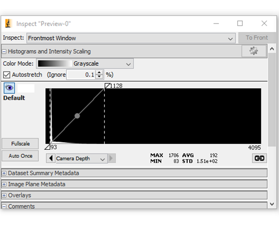
Figure 32: The 'Inspect' window. This won't appear until an image or preview has been acquired, and allows control of image handling.
It should be noted that for fluorescence or low-light imaging of sensitive samples, the signal intensity from the sample will be far lower than the maximum value the camera can display. In the example histogram in Fig.33 (copied from Fig.32) the camera can display intensities of up to 4095, but the highest signal from the sample is at 1128. The large peak at the left of the histogram (red square) represents all the black background pixels where there is no sample present, the area in the green square represents the pixels of the sample, displaying a range of intensities.
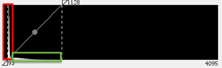
Figure 33: An example histogram from the 'Inspect' window. The red area shows all the black pixels of a fluorescence image, and the green area shows all the image pixels. The rest of the camera full-well (up to 4095) remains unused.
By changing the histogram and scaling controls you can determine how your acquired data is displayed on your screen. Please note that this doesn’t change the signal intensity from your sample, just how this data appears on your screen.
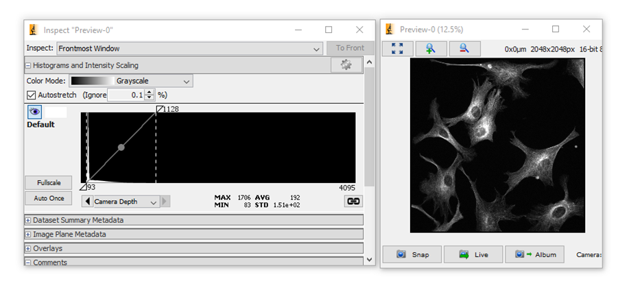
Figure 33: The 'Inspect' window with histogram, next to the image containing the histogram data (Preview-0).
By default, automatic image scaling is used to set the maximum and minimum displayed intensity values based on image data. In Micro-Manager this is called ‘Autostretch’, and is enabled by default, as seen by the tick box above the histogram. When autostretch is enabled, the scaling will automatically match to the max and min values, such as 93 and 1128 as seen on the previous example.
If autostretch is disabled, the maximum and minimum will need to be manually set for each acquisition. If the light level or exposure time are changed, the signal intensity will also change and the histogram may go beyond the manual scaling points, so if deactivating autostretch please check your histogram and image each time you change anything that may affect signal level.
As values of the very brightest and very darkest pixels can change rapidly, it is typical to ignore some percentage of the brightest and darkest pixels in determining image scaling, to avoid outliers. This is shown in Micro‑Manager as the ‘Ignore %’ and typically defaults to 0.1%. This can be manually changed, but bear in mind a higher Ignore % as shown below (of 2% in this case), will result in a higher contrast image, but with more saturated pixels. The most important thing is to get the image that is most representative of your sample while also answering your scientific questions.
It is possible to manually set the max and min display values by dragging the triangles on the top and bottom of the histogram respectively. Alternatively, double click on the min or max displayed value to type in a new value. For PVCAM cameras it is important to ensure that the lowest value is ~100, as this is the base level of offset in the camera settings.
Note: sometimes when saving an image as a .tiff from Micro-Manager and then opening in a default image viewer like Windows, it can appear completely black. This is because the image is not 'Autostretched' and you are viewing the full 12-bit well from 0 to 4095. For a fluorescence image the signal is typically on the lower end, so if using only default image viewers, save as a .png or .jpeg to bake in the histogram stretch settings (at the cost of some image compression).
Gamma
The typical way to display image values is linearly, with min scaling value mapped to 0 display intensity, and a linear increase up to max scaling value mapping to 255. However, for some images such as thick samples in brightfield imaging, this can result in either poor contrast in dark areas or completely saturated bright areas.
Gamma is a non-linear mapping of intensity values, meaning more display values can be used to give contrast to dark areas of the sample without saturating bright areas, and vice versa. To change gamma, click and drag the circle in the center of the line that connects the max and min display values on the histogram. Compare the image in Fig.33 to Fig.34 below, which has modified gamma.
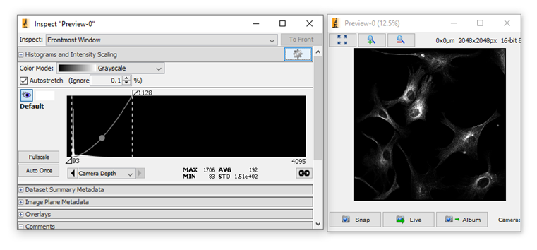
Figure 33: Image from Figure 32 with modified gamma settings. By clicking the red dot on the min/max line on the histogram, the intensity values are changed non-linearly.
Lookup Tables (LUTs)
Lookup-tables or LUTs apply false colors to image channels. The vast majority of scientific cameras are monochrome, meaning colors such as those seen in fluorescence are false colors applied after acquisition in order to differentiate between channels, such as DAPI being blue, etc.
Micro-manager comes with several LUT options for an alternative to the typical monochrome/greyscale appearance. In the above Fig.32/33 the image has a ‘Greyscale’ LUT, in the below Figure 34 the ‘Fire’ LUT is used. Different LUTs can help highlight small intensity differences in your image.
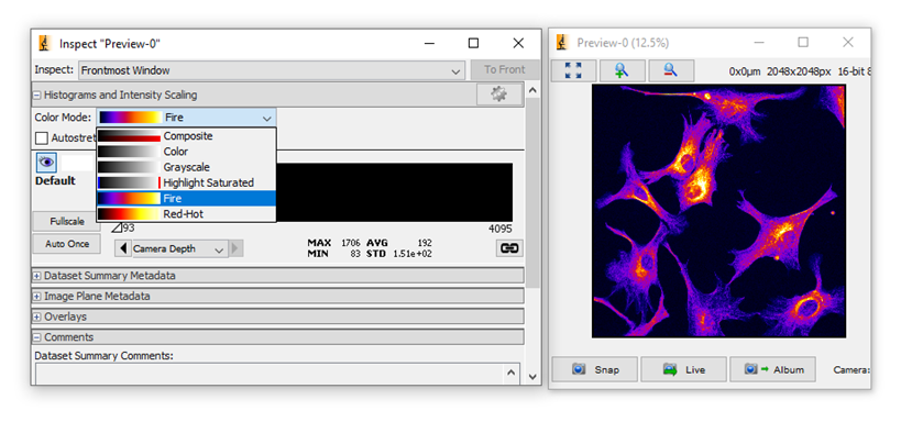
Figure 34: Image from Figure 32 with LUT changed from default 'grayscale' to 'fire'. Instead of black to white, intensities scale from purple to red to yellow.
Scale Bars
To display a scale bar in Micro-Manager, you will first need to set your Pixel Scaling Calibration, detailed in a previous section. Once set, here's how to set up scale bars in Micro-Manager:
1. In the Inspector window under the Overlays tab, click the ‘+ Add’ button, and choose ‘Scale Bar’.
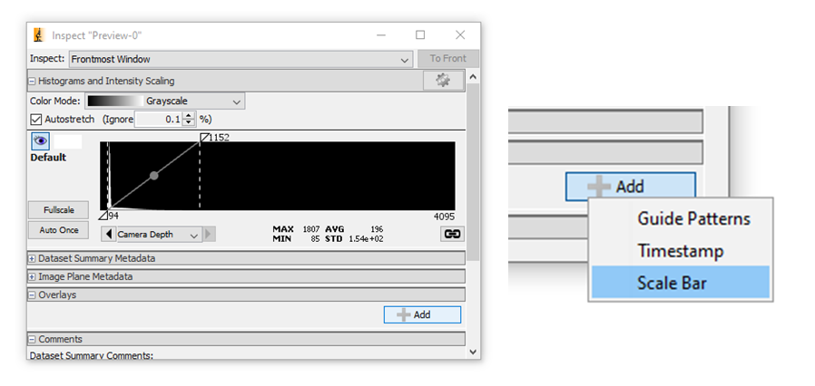
Figure 34: In the 'Inspect' window, go to 'Overlays' and select 'Add', then 'Scale Bar'
2. Multiple options for length, thickness, color, label and position are then available.
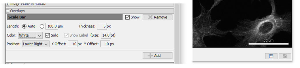
Figure 35: Options for length, thickness, color, label, positon, etc. The scale bar can be seen on the image on the right.
Regions of Interest (ROIs)
A region of interest (ROI) allows you to select the part of the camera sensor you'd like to acquire an image from. If your camera field of view (FOV) is larger than your microscope FOV, or if your sample only occupies a small part of the camera sensor, use an ROI to only acquire from the parts you're interested in. This results in faster acquisitions and smaller file sizes. Here's how to create ROIs in Micro-Manager
1. Use the ImageJ rectangle tool (Fig.36 red box) to draw on a live or snapped image, and click the blue ‘ROI’ button outlined below (Fig. 36 left green box). To return to the full field of view, click the four green arrows button (Fig. 36 right red box).
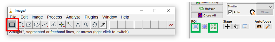
Figure 36: Once a rectangle is drawn on the image, an ROI can be established.
2. To specify an exact size and position of region of interest, use Edit / Selection / Specify… within ImageJ to specify Width, Height and X and Y co-ordinate of the top left corner. The ‘Centered’ option would instead make the reference point for the X and Y co-ordinate the center of the ROI.
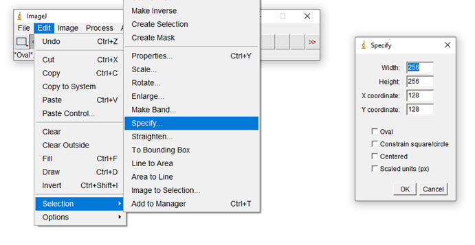
Figure 37: In the ImageJ window, go to 'Edit', then 'Selection', then 'Specify...' to open the Specify window. This lets you control your ROI to exact parameters.
3. You can also save selections to ImageJ’s ROI Manager to save them to a file and load them by dragging and dropping the file onto ImageJ, or to select between multiple ROIs.
4. Once you have drawn up your chosen ROI, click the blue ROI button outlined above to apply it to the camera.
Multi-ROI
Some Teledyne Photometrics cameras, such as the Kinetix, support Multi-ROI. Typically only one ROI can be established at a time, but if you want multiple areas of your image you want to acquire, we have developed Multi-ROI. This allows up to 16 regions to be imaged simultaneously. The overall camera readout and image size will be determined by the bounding box containing all ROIs – the camera will not skip rows not contained within an ROI. The rest of the image will be set to a greyscale value of ‘0’, which when used with lossless compression can significantly reduce file sizes, and lead to easier segmentation.
Note: Multi-ROI support requires a compatible camera and Micro-Manager version 2.0 or above. Version 1.4 is not compatible with this feature
Here's how to use Multi-ROI in Micro-Manager:
1. Draw your first ROI as normal
2. Hold shift, and begin drawing the second ROI from the top left corner. With shift held, the ROI will be constrained to a square.
3. Release shift without releasing the mouse button to draw rectangular ROIs.
4. Release the mouse button, and repeat for all further required ROIs. Note: ROIs can overlap.
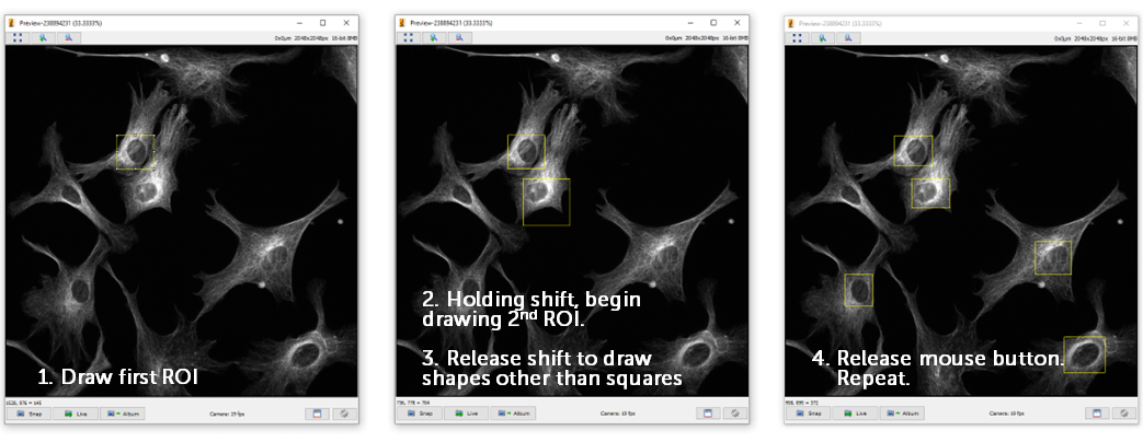
Figure 38: How to use Multi-ROI in Micro-Manager to establish multiple ROIs (up to 16).
5. Should you wish to store the ROI locations for future acquisitions, at this stage, you are able to press ‘Ctrl+T’ to add this multi-part ROI to the ROI Manager, where it can then be recalled if lost, or saved for future use.
6. Press the blue ‘ROI’ button to apply the regions as before. This will produce a Preview showing only the ROIs.
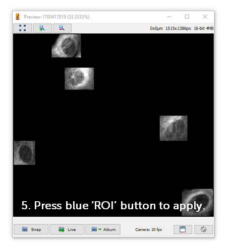
Figure 39: Multi-ROI image preview.
Multi-Dimensional Image Acquisition
Acquiring more than one frame in Micro-Manager is handled via the Multi-Dimensional Acquisition window (‘Multi-D Acq.’). This is where you can design experiments with whatever hardware you have connected – multi XY positions, Z positions, multi-channel, and of course time points for both streaming and timelapse acquisition. There is also the option for autofocus at designated times.
The Acquisition Order dropdown provides control over what order changing hardware parameters happens. For example, whether each wavelength channel is imaged sequentially on each z-slice (desirable for best co-localization), or whether the entire z-stack is acquired before changing between channels (desirable if changing wavelength channels involves time-consuming filter wheel or dichroic changes).
Setting up multiple XY Positions and Z stacks is intuitive and straight forward, but not covered in this guide. Information can be found on the Micro-Manager website's own guide: RECORDING IMAGES
The different formats of Multi-Dimensional Acquisition covered here are 'Movies & Timelapse' and 'Multi-Channel'
Movies & Timelapse
1. To acquire a movie/streaming acquisition where the camera runs at full speed (or according to external triggering control), simply set the number of frames you wish to acquire under ‘Time Points / Count’, and leave ‘Interval’ at 0.
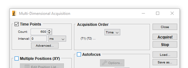
Figure 40: Acquiring a movie using Multi-D acquisition, use the 'Time Points' settings.
2. To acquire a timelapse where there is a delay between frames/stacks (including where appropriate multiple channels, xy & z positions), the ‘Interval’ corresponds to the target time between acquisitions, not to any additional added time between frames. If this interval is set shorter than the acquisition time per time point, it is ignored.
Multi-Channel
- To set up a multi-channel acquisition, ensure you have set up your Channel group as outlined previously in this guide (Multi-setting Groups section)
- Specify your channel group that controls channel hardware in the ‘Channel Group’ box.
- Click ‘New’ to add a channel to the list to be acquired.
- Under ‘Configuration’ specify which preset value of the Channel group this channel should have. You can set the exposure time for this channel, whether to include a z positioning offset correction, whether to include this channel in Z-stacks, whether to skip a certain number of time points before acquiring this channel, and finally the color the channel should appear.
- Repeat this for as many channels as you intend to acquire.
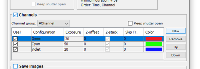
Figure 40: Acquiring a multichannel image using Multi-D acquisition, use the 'Channels' settings.
Saving Multi-Dimensional Acquisitions
By default, with ‘Save Images’ unchecked, images are acquired into RAM as usual and can be saved after acquisition.
To save to hard disk/SSD as images are acquired, check the ‘Save Images’ checkbox and specify a folder and filename. As with saving after acquisition a choice between Separate Image Files and Image Stack File is provided – Image Stack Files save faster, and hence are highly recommended for streaming acquisitions.
You will need to make sure that your computer has high enough hard disk / SSD write speed to keep up with the data rate of the camera for high-speed streaming to disk.
Image Analysis
Both Micro-Manager and ImageJ have multiple plugins and functions for live, on-the-fly analysis as well as post-acquisition analysis. Firstly, how to use ImageJ analysis.
Using ImageJ Functions & Plugins
Some ImageJ analysis functions can be used on Micro-Manager images, but some require the image to be brought explicitly across to a new instance of ImageJ. While Micro-Manager opens with an ImageJ window, this has limited functionality and lacks typical ImageJ Functions such as:
- Plot Z Axis Profiles
- Image summation & averaging
- Use of ImageJ Plugins
In order to access these and use the full suite of ImageJ analysis tools, you can open ImageJ from within Micro-Manager. This can be done by clicking the cog symbol in the Image Preview window and selecting 'To ImageJ'. Alternatively, you can manually open a new instance of ImageJ or Fiji, then open the image.
Line Profiles
To draw a line profile in Micro-Manager, use the ImageJ Line tool and then in ImageJ choose ‘Analyze / Plot Profile’. You can also use the keyboard shortcut ‘Ctrl + K’, although this shortcut will not work on a live updating image.
You can click the ‘Live’ button on the graph window that appears to have the graph live update for either an updating image or for moving the line.
You additionally have the option to thicken the line to take an average intensity measurement across the thickness of the line at each point along its length. To do this, double click the ImageJ line tool to specify line thickness.
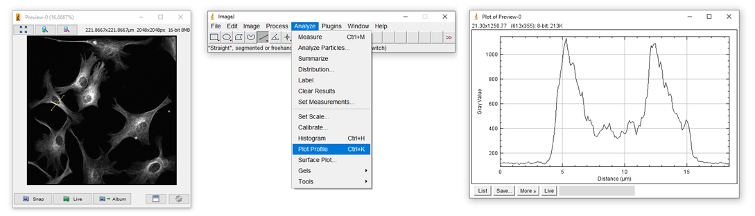
Figure 41: Establishing a Line Profile, either for post acquisition analysis or live analysis
Intensity over time and Ratiometric charts
Micro-Manager can display live intensity charts for multiple regions of interest, on either a live view or an acquiring sequence, and display a ratiometric intensity of two ROIs, for applications such as Calcium imaging.
1. In Micro-Manager, choose ‘Plugins / Acquisition Tools / Realtime Intensity Plots’. A window will appear asking you to set up ROIs. You can do this with the ImageJ ROI Manager.
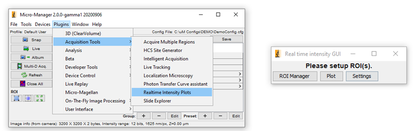
Figure 42: How to set up a realtime intensity plot.
2. To add an ROI to the manager, select your tool of choice (ROIs can be any shape) and draw an ROI, then press ‘Ctrl + T’ to add this to the Manager. You can repeat this for multiple ROIs.
3. Once all of your ROIs are listed in the ROI Manager, the ‘Real time intensity GUI’ window should show ‘Ready’. Once you hit ‘Plot’, a live updating intensity window will appear once your display is updating with live data.
4. To make a Ratiometric plot between ROIs numbered 1 and 2 in the ROI Manager, click ‘Settings’ in the ‘Real time intensity GUI’ and choose ‘Ratiometric image’.
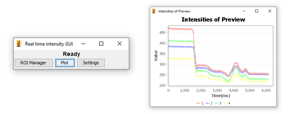
Figure 43: How to set up a ratiometric plot.
Saving and Opening Acquired Data
Files saved by Micro-Manager use the ome.tiff format, and can be universally opened in other imaging software, complete with metadata. However, Micro-Manager itself can only open files that were acquired using Micro-Manager.
Whenever you ‘Snap’, ‘Album’ or use ‘Multi-Dimensional Acquisition’ you can acquire an image, but this image needs to be saved to your storage drive if you want to open it later on. The method to save Micro-Manager files is given below. The alternative of saving via ImageJ’s ‘File / Save’ menus may not retain all metadata, and these files cannot be re-opened in Micro-Manager. Only by saving through the Micro-Manager window can you get the ome.tiff files for universal analysis.
Here's how to save acquired images to disk with Micro-Manager.
- 1. To save an acquisition, click the Save icon to the bottom right of the image (red square in Fig.44). You will be prompted to choose between two saving methods: Image Stack Files or Separate Image Files. Image Stack Files are faster to work with and can be much more convenient than separate image files for large stacks. Note: Very large Image Stack Files are split into 4GB chunks according to the maximum size of a multi‑page TIFF file. These will open as if they were one file.
- 2. Files will save in a folder according to your file name. See below for some options relating to how files are saved.
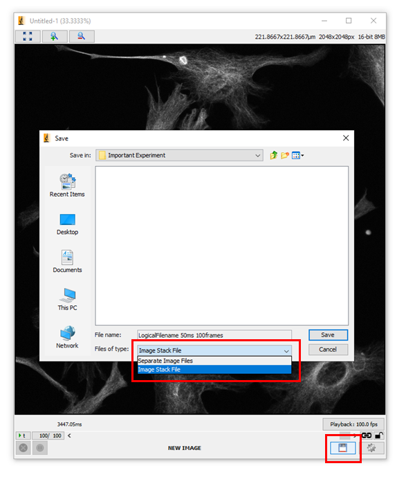
Figure 43: How to save images within Micro-Manager. Click the save icon (red square, lower right corner), then select separate files or stack (red rectangle) in the dialog.
Saving Options
The ‘Tools / Options’ menu in Micro-Manager provides access to two saving-related settings:
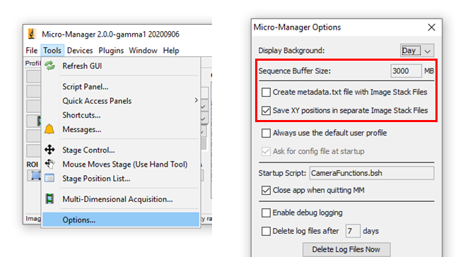
Figure 44: Go to the 'Tools' and 'Options' within Micro-Manager to access save options.
- ‘Sequence Buffer Size’ – determines how much RAM is allocated to store images before saving. If Micro-Manager is crashing during large acquisitions (1000s of frames) you may need to increase this. The value is MB so the 3000 MB in the example is only 3 GB of RAM.
- ‘Create metadata.txt file with Image Stack Files’ –stores the image metadata separately, which provides easier access to post-acquisition analysis pipelines
- ‘Save XY positions in separate Image Stack Files’ –separates XY stage positions in an acquisition into separate stack files. Note: Irrespective of this setting, when saving Separate Image Files, these files will be separated into folders according to XY stage position.
Loading images saved from Micro-Manager
- Loading images can be done via Micro‑Manager’s File menu
- Either choose Virtual access where each frame/stack slice is loaded on demand from the hard drive, or RAM access where the entire image stack is pre-loaded into the RAM. RAM loading leads to faster image access, but large stacks will require large amounts of RAM.
- Alternatively, you can open files by dragging either the tiff file or the folder containing it onto the Micro-Manager window.
- By default, this will load images into RAM, unless there is insufficient RAM in which case you will be prompted to open virtually instead.
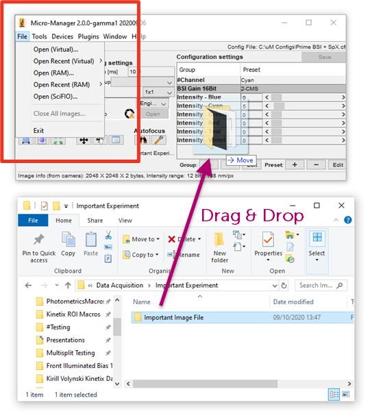
Figure 44: Go to the 'File' and 'Open' within Micro-Manager to access load options.
Streaming to RAM or Disk for High-Speed Imaging
Acquiring and saving individual files or small stacks is easily done through Micro-Manager, whether using RAM or Disk. However, with larger and faster cameras continually in development, it is important to know the limitations of Micro-Manager when streaming data to RAM or Disk at high-speeds, working with large fields of view, or doing high-throughput imaging in general.
This section mostly applies to our Kinetix sCMOS camera, which has a far higher speed and larger field of view than other scientific cameras, and consequently has a much higher data rate.
The Kinetix has a 3200 x 3200 pixel array, meaning every acquired frame has a file size of 10 or 20 MB when using 8-bit or 12-/16-bit modes respectively. When using the 8-bit speed mode, the Kinetix can acquire 500 frames a second, and with each frame being 10 MB this results in a data rate of ~5 GB/s. When imaging close to or at this data rate, Micro-Manager can struggle. This section outlines how to stream to RAM or Disk at these high speeds when using Micro-Manager.
Streaming to Disk
For the Kinetix, 12-bit 'Sensitivity' and 16-bit 'Dynamic Range' modes are able to stream at full speed to disk, allowing for constant acquisition as long as the disk still has capacity to store each frame.
But, due to limitations in the internal architecture of Micro-Manager, it currently isn't able to match the full speed of the Kinetix in 8-bit 'Speed' mode while streaming to disk. When testing computers (that met our specifications) for full-speed streaming to disk, our engineers have found a data rate limit of ~1.5-2 GB/s when writing to disk (the full data rate of the Kinetix in ‘Speed’ mode is 5 GB/s). In order to successfully stream to disk with a Kinetix at full speed when using Micro-Manager the data rate must therefore be limited, either by using regions of interest to reduce the frame size, or by reducing the frame rate by increasing exposure or using external hardware triggers.
Note: One of the reasons for a data rate limit within Micro-Manager is due to the nature of ImageJ and Java. Micro-Manager runs through ImageJ, which itself is based on Java. Every image acquired in Micro-Manager needs to be copied across to the Java backend, this requires substantial bandwidth and essentially limits the top data rate of Micro-Manager due to its architecture, and several other reasons outside the scope of this guide.
We are currently working on a solution to enable full-speed streaming to disk in Micro-Manager. In the meantime, for streaming to disk with a Kinetix in 8-bit 'Speed' mode, please contact us for an alternative free solution developed by Teledyne Photometrics.
Streaming to RAM
On a computer that meets our recommended specifications, Micro-Manager is capable of streaming to RAM (memory) at the full speed of the Kinetix in all modes. However, not all of your PC's RAM is available to Micro-Manager for acquisitions, typically ~40-50% of the available RAM is accessible.
If using a computer with 64 GB of RAM, the Kinetix may be able to stream ~32 GB of data uninterrupted. If imaging at the full 500 fps speed of the Kinetix, at 10 MB per frame, this 32 GB of RAM represents ~7 seconds of constant acquisition (5 GB/s max data rate). If using the slower 12-bit 'Sensitivity' or 16-bit 'Dynamic Range' modes at 20 MB per frame, the 32 GB of RAM represents ~18 seconds of constant acquisition.
Here's how to stream to RAM with Micro-Manager:
- Installing the correct version of Micro-Manager: Streaming to RAM will function optimally when using the latest nightly build of Micro-Manager 2.0.0 or above, please use a version dated from the 4th of March 2021 onwards. If you are constrained to use particular versions of micro-manager due to limited compatibility with other hardware, please contact us.
- Installing the Kinetix into Micro-Manager: For instructions on installing the Kinetix (or other high-speed PVCAM cameras) into Micro-Manager, please consult the relevant section of this guide.
- Setting the Sequence Buffer size: Once you have Micro-Manager installed and your required hardware configured, there are a few settings to enable high speed acquisition to RAM. The first is the Sequence Buffer Size, found within Micro-Manager under Tools -> Options. The sequence buffer holds frames that come from the camera before they are copied to and processed by the Java environment (lmageJ). At its full field of view, the Kinetix is delivering frames to the buffer up to every 2 ms (at 500 fps), but the copying to Java takes longer than this, so the sequence buffer will fill up while frames wait to be copied. The capacity of the sequence buffer can be set via Micro‑Manager in the image shown. The default size of the buffer is 250 MB, and with single snaps or slower multi-D acquisitions the buffer is not used at all, with images copied to Java directly. To maximize the possible acquisition data size. the sequence buffer should be set to ~40-45% of available computer RAM. For a given acquisition size the sequence buffer should be set to a similar size. If your available PC RAM isn’t sufficient, the buffer can overflow and acquisition may fail, which will produce an error message.
- Setting the ImageJ Memory size: After being stored in the sequence buffer within Micro-Manager, your images are copied to ImageJ for processing, displaying, or saving to disk. This means you also need to consider the memory size allocated to ImageJ itself. The memory size can be set via lmageJ -> Edit -> Options -> Memory & Threads. To maximize the possible data acquisition size. the lmageJ maximum memory should be set to ~45‑50% of the computer's RAM, similar to the amount allocated to the sequence buffer. With ~40% RAM allocated to the Micro-Manager sequence buffer, and ~40% RAM allocated to the ImageJ memory, your PC has 20% of its total RAM left for the operating system and any other open programs to run. To see how much RAM your computer is using, and what it is being allocated to, right-click the windows button and select ‘Task Manager’. There will be columns for CPU, Memory, Disk and Network. The ‘memory’ column is your computers RAM, and the percentage shows how much of it is in use. If more than 20% of your RAM is being used before you even open Micro-Manager, you may need to close some programs, especially RAM-hungry programs like Google Chrome. If you don’t know how much RAM your computer has, click the ‘Performance’ tab within the Task Manager and go to ‘Memory’, this will show you how much memory you have, and what is currently in use.
- Running an Acquisition: Set up your experiment in Micro-Manager as normal. When setting up your large acquisition through the Multi-Dimensional Acquisition window you will see the ‘total memory’ for the acquisition updating as you fill in the fields. For example, this acquisition will require ~8.8 GB of memory. This should be less than the memory given to ImageJ in step 4, and roughly the same as the sequence buffer size given to Micro‑Manager in step 3.
Monitoring Image Acquisition
If you are acquiring at high speed, the sequence buffer is expected to fill up very quickly. This can be monitored via Micro-Manager -> Plugins -> Developer Tools -> Sequence Buffer Monitor. This should not reach 100% during acquisition.
Java memory utilization can also be monitored: lmageJ -> Plugins -> Utilities -> Monitor Memory. Similarly, this should stay below 100%.
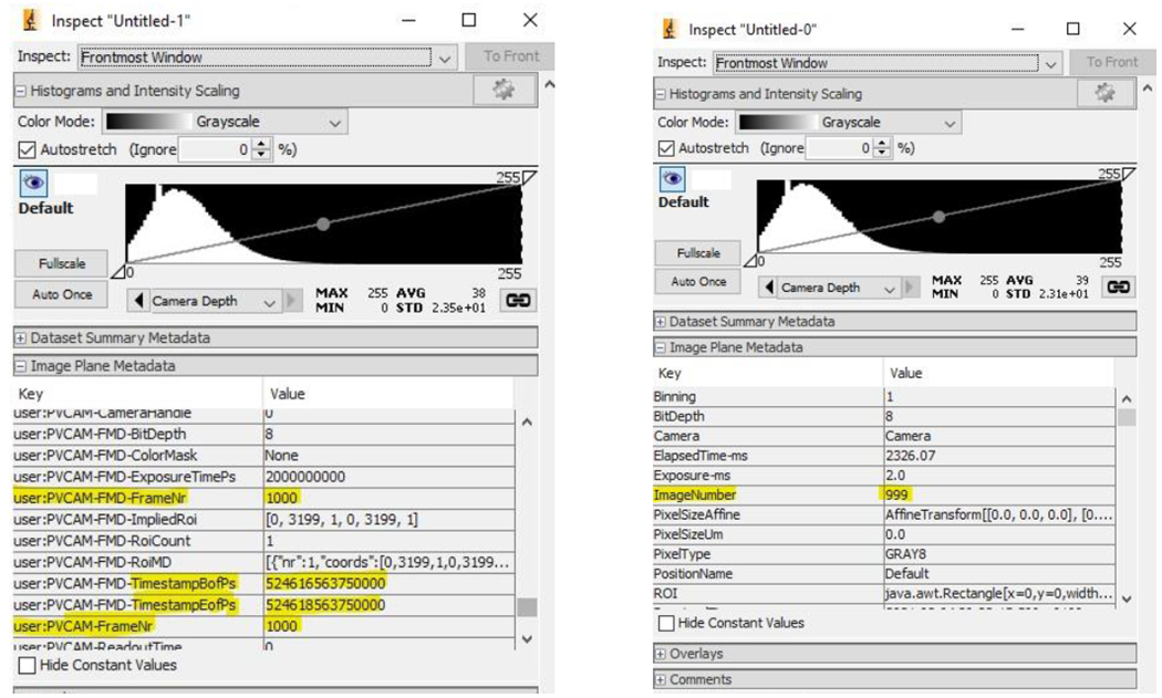
Once an acquisition has completed, select the Inspect window in Micro-Manager and open the 'Image Plane Metadata' section. The total frame values in ‘PVCAM-FMD-FrameNr’ and ‘PVCAM-FrameNr’ should be the same. This should also be one greater than the ‘lmageNumber’, as the first frame has a lmageNumber of 0.
If the metadata frame numbers are larger than your requested number of frames, frames were acquired by the camera that the computer was not able to record, and those frames are lost. To avoid frame losses, you may need to reduce the total acquisition size or reduce the acquisition speed or data rate.